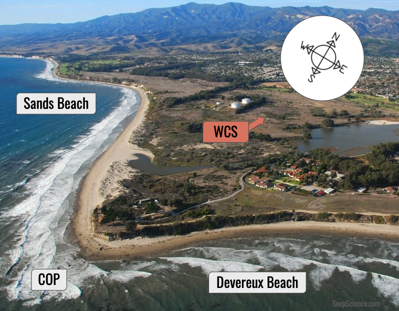
The study “Long-Term Atmospheric Emissions for the Coal Oil Point Natural Marine Hydrocarbon Seep Field, Offshore California” by Ira Leifer, Christopher Melton, and Donald R. Blake was recently published in Atmospheric Environment and presents a novel method for deriving atmospheric emissions from natural marine seepage. The study analyzed three decades of air quality station data using a Gaussian plume inversion model. Specifically, total hydrocarbon concentration and meteorology data from West Campus station (WCS), which is an air quality station proximate to and onshore from the Coal Oil Point (COP) seep field. The study found seep field hydrocarbon gas atmospheric emissions of 83,500±12,000 m3 day-1, for a three decade average (1990-2021).
This study presents the first directly-inferred atmospheric emissions from a seep field (as opposed to deriving seabed emissions and estimating atmospheric emissions by a numerical model to predict the air / ocean partitioning). It also is based on the longest dataset to date, by far. The approach leveraged WCS, which is 2 km from the seep field, onshore from Coal Oil Point. Field air samples show that methane is overwhelmingly the predominant hydrocarbon gas (>95% of the hydrocarbon gases emitted).
Methane and Natural Seepage
Although only some marine seeps release both oil and gas, most marine seeps release gas, primarily methane, which escapes from subsurface reservoirs through faults and fractures in the overlying rock and sediment layers. Methane is a potent greenhouse gas, far more potent than carbon dioxide on a per molecule basis. Because of its importance to the atmospheric radiative balance, and shorter lifespan (decadal) than carbon dioxide, there is strong interest in methane regulation; however, this requires a good understanding of the contribution from (unregulatable) natural sources including geological sources. Assessing geological emissions is highly challenging as they are very unevenly dispersed and often located in an oil production field – assessing emissions for marine geological seepage is even more challenging given the difficulty of working at sea. Moreover, a field survey only provides a snapshot, which may be unrepresentative – particularly for a phenomenon that varies significantly on timescales from seconds to decades.
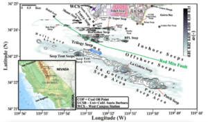
Sonar return map of the COP seep field. WCS labeled with a purple star.
The present study’s novel application of an inversion Gaussian plume model – essentially asked the question: What are the seep field emissions that can explain the observations (concentration for a given wind speed) at WCS?
The Gaussian plume model assumes a point source atmospheric plume, yet the seep field is an area source. This was addressed by gridding the seep field based on a sonar map into many small cells, each with its own Gaussian plume, which is approximated as a point source. We tested this approximation with field data, which showed that emissions from areas of intense seepage (i.e., less than a grid cell) were Gaussian. Each grid cell’s plume is calculated, rotated into the wind direction/ grid cell direction (which are the same by definition), and all plumes are added together. This calculates a wind direction profile of concentration at WCS – different wind directions allows WCS data to “probe” different seep field areas. This comparison between observed and calculated is used to adjust each grid cell’s emissions and the process repeated until convergence.
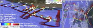
A) Methane concentration and winds data. B) Methane concentration and winds displaying the concentrations of the Gaussian plume inversion model for Trilogy Seep (lower middle). Sonar return map shown on the sea surface.
The three-decade (1999-2021) average seep field-wide atmospheric THC gas emissions were 83,500±12,000 m3 THC day-1 (~3 million cubic feet per day). THC is total hydrocarbon. However, approximately half the seabed gas dissolves (based on a study by Clark et al.) and thus does not reach the atmosphere. This implies seabed emissions of 167,000 m3 THC day-1 (~6 million cubic feet per day). Seep seabed emissions are split between the atmosphere and water column and depend on seabed depth and emission character – emissions can result in bubbles, bubble plumes, or dissolved methane with bubbles slowly dissolving while rising through the water column.
The study’s estimated seabed emissions of 167,000 m3 THC day-1 is similar to a prior estimate of COP seep field seabed emissions by Hornafius et al. (1999), 150,000 m3 dy-1. This agreement is coincidental as concentrations varied significantly over the decades indicating higher emissions time, when concentrations are higher. Moreover, the Hornafius study was for late summer and fall 1994-1996, when concentrations were at a minimum. Another sonar survey by Padilla et al (2019) in late summer/fall of 2016 estimated a much lower 24,000 m3 day-1, which arose in part from field subsampling, calibration issues, and seasonality. Note, neither of these studies addressed seasonality – both Hornafius and Padilla sonar surveys were in the summer and fall, when seepage is at a minimum, whereas winter and early spring have much higher seepage due to storms. This study’s estimate includes data for all seasons, including storms, large transient events, and even emissions from outside the mapped seep field extent.
Emissions Variability
WCS data displayed patterns of THC concentration that varied daily, seasonally, and yearly. Winds follow a diurnal (daily) cycle – blowing towards shore during the day, and offshore at night. This wind pattern results in higher THC at WCS in the morning and late evening hours. Seasons also change the temperature and weather patterns that affect seep gas emissions. January had the highest emissions, while July had the lowest. These seasonal trends closely followed onshore wind patterns further confirming that wind patterns largely account for changes in seep emissions.
This new study was conducted by BRI in collaboration with the Donald Blake Laboratory at UCI, who analyzed air samples to determine the composition of the seep air emissions. Emissions mainly were composed of methane, carbon dioxide, and ammonia. In addition, the survey explored the presence of non-methane hydrocarbons that are typically released alongside methane from underground hydrocarbon reservoirs. The most common non-methane hydrocarbon in the emissions sample was ethane. Carbon Dioxide was associated with oil field infrastructure, and the hydrocarbons (including methane) are emitted from the oil and gas underground reservoirs.
Related Articles
-

California Scientists Develop New Tool to Understand Dairy Air Quality
-
SISTER2 Summer Field Campaigns with NSF, NASA, & CEC
-

Volcanic Gas Discovery leads scientists to investigate the potential for Active Magma Reservoir Under Death Valley
-
Featured Article – SIS™: A “Science Cube” developed for off-road data collection